Modeling Strikeout Rate with Plate Discipline Part 1: Hitters

Strikeout and walk rates are perhaps the most popular and widely used peripheral statistics, particularly for pitchers. However, with pitch level data, these statistics now have “peripherals” of their own. I was curious if I could create an accurate yet interpretable model using FanGraphs’ plate discipline metrics that could offer insight on what drives the differences in strikeout and walk rates between players. For the first part in this study, I will focus on hitter strikeout rate, but I intend on also looking at walk rate and, later on, pitchers’ strikeout and walk rates.

Methodology

Note: I used BIS discipline statistics rather than PITCHf/x. I do not think this made a significant difference, but I think it is important to keep in mind.

FanGraphs gives us 9 plate discipline statistics to work with. However, several of them can be removed as they can be derived using the other statistics. In a regression setting, this phenomenon is called perfect multicollinearity, which is when an explanatory variable can be perfectly formulated by a linear function of other explanatory variables. Multicollinearity is a problem for inference because with a high degree of multicollinearity, it can be extremely difficult to tell which particular variable is responsible for a change in the response variable. In this context, Swing%, Contact%, and SwStr% are all examples of perfect multicollinearity. While they provide useful overviews for plate discipline, I would rather use their components for a regression to maximize the data’s information. An imperfect analogy is OPS. While OPS is a better overall offensive metric than either on-base or slugging percentage, I would rather have both on-base and slugging rather than OPS for more information on the hitter. Using some basic dimensional analysis, I found formulas for all three of these:

• Swing% = O-Swing% * (1 – Zone%) + Z-Swing% * Zone%
• Contact% = (O-Contact% * O-Swing% * (1 – Zone%) + Z-Contact% * Z-Swing% * Zone%) / Swing%
• SwStr% = (1 – O-Contact%) * O-Swing% * (1 – Zone%) + (1 – Z-Contact%) * Z-Swing% * Zone%

Note that while the formula for Contact% uses Swing%, you can simply plug in the formula for Swing% here to have a formula in terms of the other variables. After figuring out these formulas on paper, I also verified them with R.

Now we are down to 6 variables. At this point, I had a question; how quickly does each variable provide meaningful information about a hitter? To answer this, I did an informal check by looking at correlations between the first and second half values of these statistics using players from 2015 through 2019 who accrued at least 250 and 200 PA’s in the first half and second half respectively.

Statistic	First-Half to Second-Half Correlation
O-Swing%	0.827
Z-Swing%	0.833
O-Contact%	0.812
Z-Contact%	0.786
Zone%	0.664
F-Strike%	0.463
K Rate	0.794
BB Rate	0.713

I want to emphasize that this is a non-ideal way to figure out the information different statistics provide. For example, the correlation method doesn’t account for any potential plate discipline erosion that occurs over the season. For a better approach, I would check this out. However, for our purposes, I think it gives us a rough idea of the information the statistics provide. For the first four variables, it appears that, at the very least, they provide equal if not better information than either strikeout or walk rate given equal plate appearances. On the other hand, zone and first-pitch-strike rate seem to provide less information given equal plate appearances than the other statistics. I will still experiment with them in the regression, but these correlations will definitely impact and qualify my interpretations.

Next, I created the data set for the regression, using all player seasons from 2012 through 2019 with at least 400 PAs. I chose 2012 as my starting point for several reasons. Firstly, it was the first year that strikeout rate began to increase league-wide. I was worried that if I went too far back, the strikeout environment would be too different from recent years and perhaps couldn’t be modeled in the same way as current day. However, I still wanted to have as much data to build my model as possible, so I felt that 2012 was a good compromise as a cutoff year. I chose 400 PA’s somewhat arbitrarily, but I thought it was a good cutoff point as the reliability for both strikeout and walk rate are above 70% and 400 is still a low enough limit to create a fairly large dataset. There were 1657 player seasons that met the above criteria.

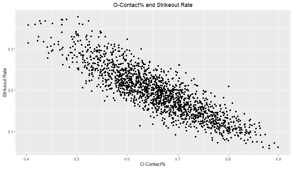
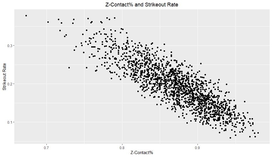
Before splitting my dataset, I looked at the individual correlations between the variables and strikeout rate. The two highest were Z-Contact with -0.851 and O-Contact with -0.868. Hopefully, my model will be able to significantly outperform both of these two variables on their own.

Next, I randomly divided the observations up, giving 1000 to my training set, 300 to my cross validation (CV) set, and 357 to my test set.

In addition to my main terms, I also tested 4 interaction terms and polynomial terms up to the third degree for every variable. When formulating possible interaction terms, I thought that the swing, contact, and zone variables could have a potential synergy effect. For example, if a hitter swung a lot out of the zone AND also didn’t make much contact on swings out of the zone AND received a lot of pitches outside of the strike zone, it makes sense that this hitter may have a higher strikeout rate than one would assume from simply looking at O-Swing%, O-Contact%, and Zone% independently. This brings me to an important change I made: I used O-Miss% = 1 – O-Contact% instead of O-Contact% and Non-Zone = 1 – Zone% instead of Zone% in order to consider some of these interaction effect. Overall, I tested O-Swing * O-Miss, O-Swing * O-Miss * Non-Zone, Z-Swing * Z-Contact, and Z-Swing * Z-Contact * Zone. I also mean-centered my main terms to help interpretability and lower multicollinearity introduced by the polynomial and interaction terms.

Generally, whenever you include interaction terms in a regression, you also keep the individual terms that compose the interactions, even if they aren’t particularly helpful for the regression. However, because Non-Zone% and Zone% are redundant, I just used Non-Zone% in my regressions instead of including both.

Lastly, I wanted to discuss the several regression methods I modeled with. I used standard multiple regression, the lasso, and ridge regression. To implement the lasso and ridge regression, I used the glmnet R package. To select a value of lambda, I used cv.glmnet() and supplied a range of lambda values to perform cross validation on. Big shout out to the authors of ISLR. Their sample code in the textbook was an excellent reference for me and ISLR is also an excellent way to learn about statistical learning for those interested.

If you have any more questions on my methodology, you can either comment, tweet at me, or check out my Github. However, because this is an ongoing series, I probably will not update my Github with the code for this project until the whole series is done.

Results

Model 1

I will share the results of two models. The first model is the basic multiple regression with only main effects, minus O-Swing%, which I omitted due to its small coefficient and limited improvement to the cross validation mean squared error (CV MSE).

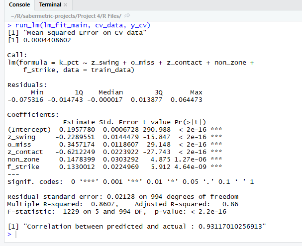
While this model did not have the lowest CV MSE, it was in the ballpark of the best MSE and also was the simplest and most interpretable model. Below, I compared this model to two simple linear regression models based on O-Contact and Z-Contact, as they were the two explanatory variables that correlated the most with strikeout rate.

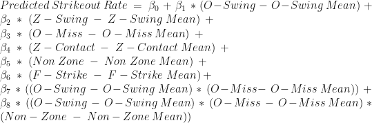
The overall formula is:

with the below values:

Variable Name	Training Data Mean	Coefficient Name	Coefficient Value (Rounded from above output)
Intercept	NA		0.196
Z-Swing	0.6745		-0.229
O-Contact	0.6603		0.346
Z-Contact	0.8702		-0.621
Non-Zone	0.5661		0.148
F-Strike	0.5986		0.133

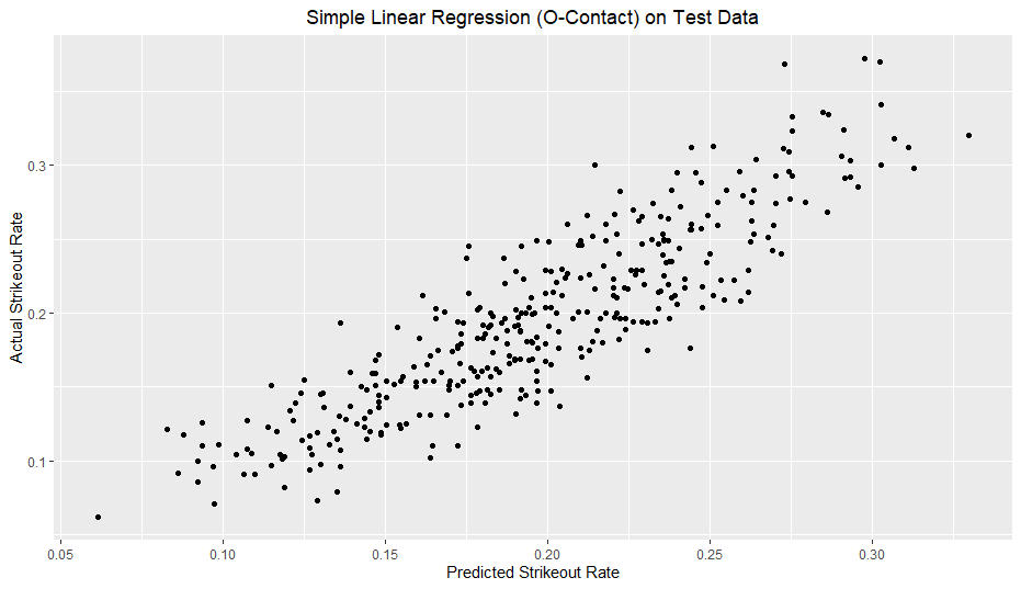
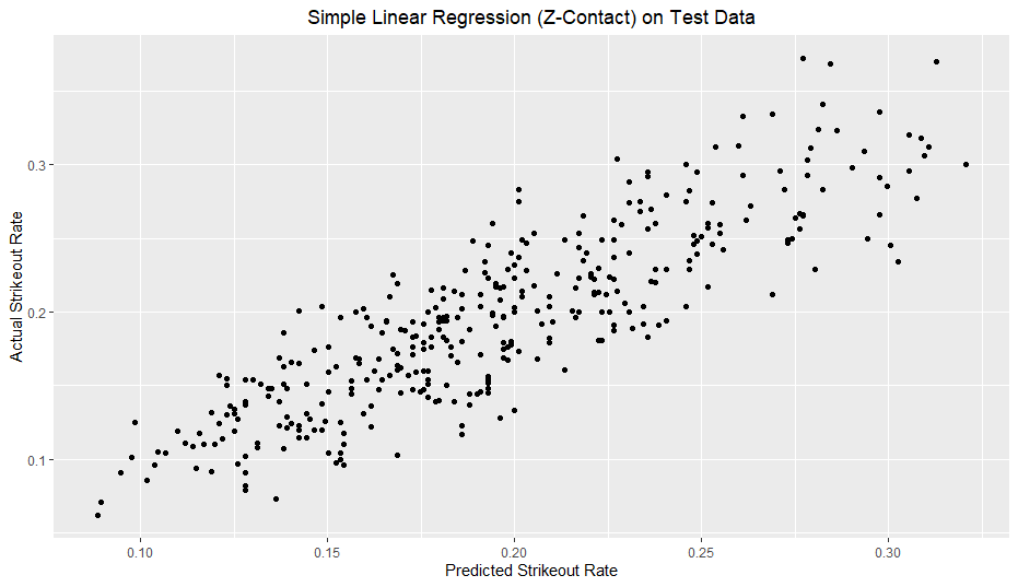
As you can see, the main-effects only multiple regression far outperformed models solely based on O-Contact and Z-Contact, with test MSE’s roughly double for the simple linear regression models.

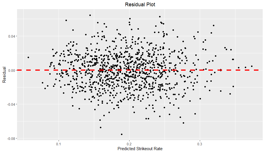
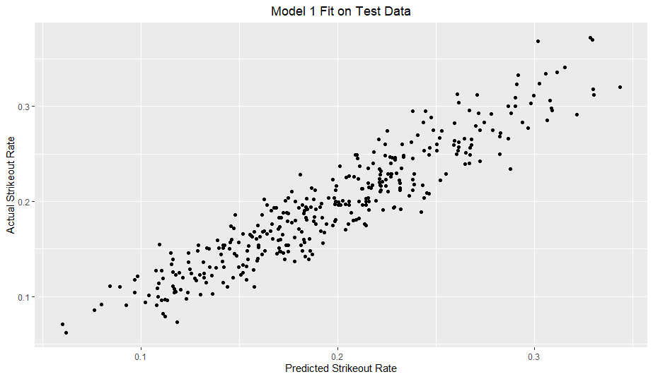
The residual plot seems to be quite random and scattered with little evidence of heteroscedasticity, but the model fit on the test data shows some very slight heteroscedasticity for high values of strikeout rate.

Next, here is the model with the best (roughly) CV error. While a few other models had slightly lower CV errors, I chose this one as it was the simplest in that group and had low p-values for all of its terms. However, I do want to mention that even though it has the lowest CV error (again, roughly), it is not significantly lower than the above model and secondly, the interaction terms make it harder to interpret.

Model 2:

The overall formula for Model 2 is:

Variable Name	Coefficient Name	Coefficient Value
Intercept		0.196
O-Swing		0.054
Z-Swing		-0.246
O-Miss		0.357
Z-Contact		-0.628
Non-Zone		0.108
F-Strike		0.094
O-Swing * O-Miss		0.294
O-Swing * O-Miss * Non-Zone		-8.582

The training data mean for O-Swing is 0.3087 and the rest of the means are in the previous table.

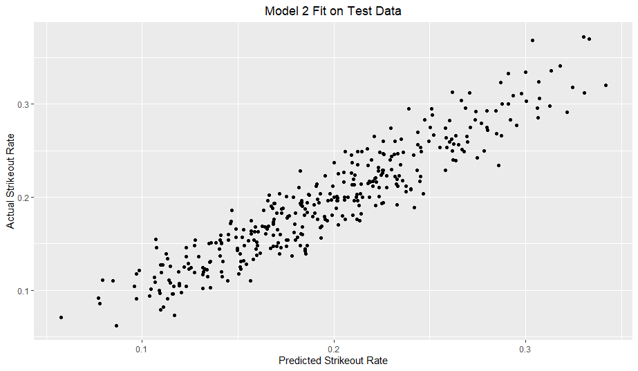
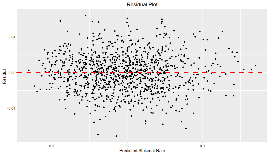
This residual plot also seems quite randomized, and the slight heteroscedasticity in the fit seems even more minor here.

Additionally, I chose not to include any of my lasso or ridge regression models. Neither outperformed standard multiple regression in terms of CV MSE.

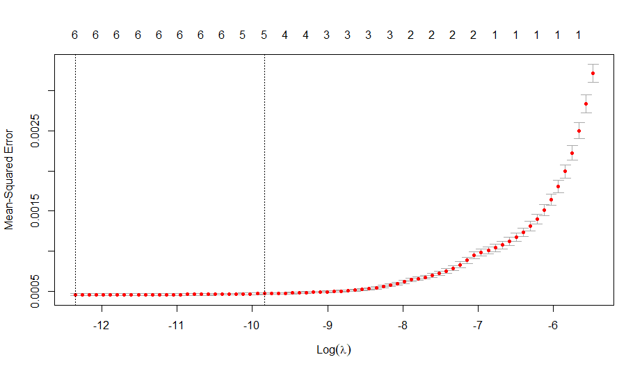
As you can see, the tuning parameter lambda seemed to produce the smallest MSE for the values closest to 0 and when lambda equals 0, both lasso and ridge regression just become standard multiple regression. This graph was generated with cv.glmnet()’s default lambda values which can be very odd, but when I tested with my own lambda list, 0 was often chosen as the ideal lambda. In other words, 0 (or close to 0) seems like the ideal value of lambda, which means both lasso and ridge regression don’t provide much over standard multiple regression. Because I had a relatively high number of observations and relatively few predictor variables, all of which seemed to have linear relationships with the response, it makes sense that there was little overfitting for the lasso and ridge regression to correct.

Lastly, for both models, all terms, including interactions, had VIF values all well under 5, which is great from a multicollinearity perspective.

Analyzing Interaction Terms

Before getting into my overall interpretations and conclusions, I wanted to analyze the interaction terms in my second model.

Two Term Interactions

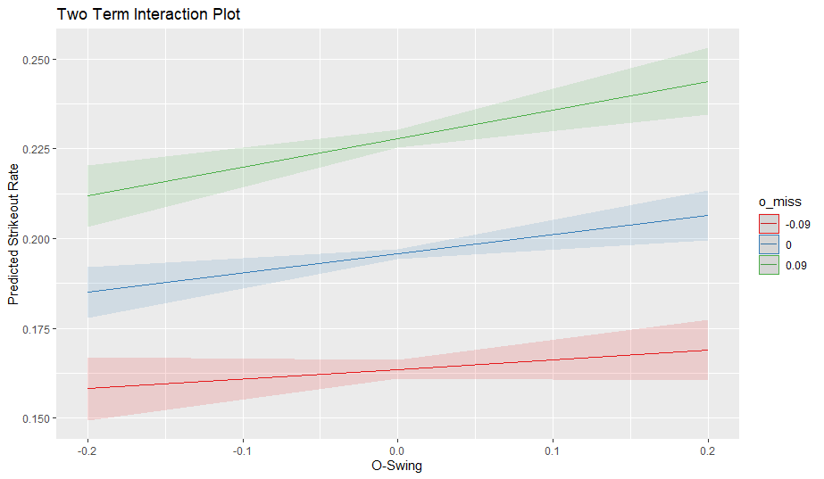
The above graph is perhaps the most significant result of my entire project. I created this graph using the sjPlot package. In this graph, the green, blue, and red lines correspond to the value of O-Miss one SD above the average, the mean value of O-Miss, and the value of O-Miss one SD below the average respectively. Notice that the mean of O-Miss is zero, as I mean-centered all the main effects. As you can see, for a higher value of O-Miss, the corresponding increase in predicted Strikeout rate accompanying an increase in O-Swing is larger, shown by the slope in each line. Even though the starting point of the green line is highest, it also has the steepest slope of any lines. On the other hand, when O-Miss is small, the slope is smaller, meaning that a larger O-Swing boosts the predicted strikeout rate less than a simple linear model would expect. Essentially, Model 2 suggests that there is a synergistic relationship between O-Swing and O-Miss, as I suspected. However, the p-value, while under the general 0.05 threshold, is not minuscule, so I would not say that this relationship exists with certainty.

On the other hand, the Z-Swing * Z-Contact interaction term showed little evidence of existing in the training set, which is why I omitted it from Model 2.

Three Term Interactions

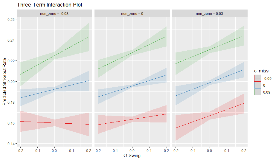
While the training data gave evidence for the O-Swing * O-Miss * Non-Zone interaction term, its third dimension makes interpretation much more difficult.

Looking at this data, I really cannot see a unifying interpretation. The slopes seem to equalize as you go from the left to right graph, possibly indicating that the O-Miss * O-Swing interaction term is stronger for lower values of Non-Zone (i.e. more pitches in the strike zone), but I’m not really sure why that would be. I also found the red line in the far left facet interesting. Essentially, for hitters who get a lot of strikes and do not miss on pitches out of the zone too much, O-Swing really does not affect Strikeout Rate for this model very much. This does make some sense, as these hitters deal with fewer pitches out of the strike zone and also make contact on those non-zone pitches more often so the effect of their O-Swing is minimized. Feel free to share any observations you can see from the above graph. The p-value for this interaction term is also not exceedingly small and because of its lack of intuitive reasoning, I would treat this term with even more skepticism.

Similarly to the two-term interaction, the Z-Swing * Z-Contact * Zone interaction term showed was not statistically significant in the regression and did not meaningfully lower the CV MSE.

Interpretations and Conclusions

There are three fairly basic and obvious interpretations I’ll mention briefly:

• Swinging and missing in and out of strike zone generally increases your strikeout rate
• Swinging more in the zone generally lowers your strikeout rate
• Both of my models far outperformed simple linear regression models based on O-Contact and Z-Contact, the two main effects most directly linked to Strikeout Rate, on the test set

I find these two points more interesting:

• More pitches in the zone generally corresponds to a lower strikeout rate
• More first pitch strikes correspond to a higher strikeout rate

As I noted in the methodology section, Zone/Non-Zone and especially F-Strike had lower first-half/second-half correlations than the other variables. Zone still had a 0.664 correlation, which makes me suspect that there is some predictability in a hitters Zone%. Specifically, I wonder if a higher Zone% is not causing lower strikeout rates but rather is a reflection of pitcher’s perception of the hitter as a dangerous or strikeout-prone hitter. For example, by 2015, most pitchers should know that Ben Revere is not a particularly strikeout prone or intimidating hitter. Thus, he received more pitches in the strike zone than most hitters. In other words, Zone isn’t causing a change in strikeout rate; rather it could partially reflect the general perception of a hitter’s strikeout ability from prior data, which ends up making Zone a useful predictor in what the strikeout rate “should” have been. Zone, rather than being an independent variable in the regression, could be a crude estimation of past strikeout rate, although there could be hitters with low strikeout rates who chase a lot and are thus given fewer pitches in the zone. However, this is conjecture and the project’s limited scope does not really give us insight on what drives Zone% for hitters.

With F-Strike, I think some of my conjecture on Zone could be applied here but with only a correlation of 0.463, it doesn’t seem as stable or interesting to me. I will say, though, I did not expect F-Strike to play much of a role at all. I underestimated the effect a first pitch strike can have on the overall trajectory of a plate appearance.

• O-Swing does not, as a standalone variable, contribute very much to a linear model.

While O-Swing did play a role in interaction terms, it individually did not have a large effect in my models. It seems somewhat counterintuitive, as you would expect that swinging at balls would correspond with a strong increase in strikeout rate, whereas I found that the increase was very small. However, you can be a free swinger and maintain a low strikeout rate if you make enough contact, like Jose Iglesias for example. Conversely, Z-Swing had a much stronger effect on strikeout rate, which muddles things up somewhat.

• There is evidence for the interaction terms O-Swing * O-Miss and O-Swing * O-Miss * Non-Zone being meaningful

Both of the above terms were statistically significant using the coefficient p-values (under 0.05), but not overwhelmingly so. I think these findings warrant further study, particularly for the O-Swing * O-Miss term, as it also has a reasonable interpretation.

Conversely, Z-Swing * Z-Contact and Z-Swing * Z-Contact * Zone had little statistical evidence for existing in the actual model.

• Polynomial terms had no statistically significant evidence for any variables

Both in terms of p-values and CV MSE, I could not find any evidence for polynomial terms up to the third degree for any explanatory variable.

Limitations

While I think this project had some interesting findings, there are several limitations I wanted to bring attention to.

• Plate Discipline does not consider the ball-strike count

FanGraphs’ plate discipline metrics treat every pitch equally; however, in a real plate appearance, the count matters tremendously. While I haven’t personally verified it, it is very likely that plate discipline changes within certain counts, like Joey Votto choking up with two strikes. Treating a swing and a miss in an 0-0 count versus a two strike count equally is not ideal, but it is the reality when working with these metrics.

• Bias with Multiple Regression

As the lasso/ridge regression tuning parameter graph showed, overfitting did not seem to be a major issue. However, I do think underfitting could be a problem with a simple, inflexible model like multiple regression. While fitting various models, I noticed that adding interaction terms, even ones with large standard errors and high p-values, nearly always reduced the CV error, even if only marginally. I do think that using a more flexible method, such as splines, would perform better from an MSE/performance perspective, but I am happy with the interpretive value multiple regression gave for this project.

• Descriptive rather than Predictive

An important asterisk on my models is that they are not meant to be predictive. Firstly, several of the explanatory variables, namely Zone and F-Strike, are not extremely stable as shown in my rudimentary correlations earlier. Even though they added value to my models, they are not stable enough to extrapolate an input from the models as a baseline strikeout rate going forward. Secondly, these models do not take into account age, changes that come about due to change, etc. Lastly, related to my previous point, these models were built to balance interpretation and accuracy, not maximize accuracy, so I would not recommend using it in a predictive way, even if you ignore the above reasons.

• Assumption of Underlying Model Consistency

Because I used data from 2012 onwards, I’m implicitly assuming that the underlying hitter strikeout model is consistent despite various league hitting trends. If this assumption was not true, the validity of my results would be questionable. However, even with the large but not drastic leaguewide shifts, I see no reason why the underlying model would change significantly, especially in regards to inference. Swinging and missing more should be linked to more strikeouts, regardless of the environment. While different environments could make swinging and missing less impactful, the overall inferences from my models should not drastically swing from year to year.

What’s Next?

As I said earlier, I intend on using this same methodology for hitter walk rate and later on, looking at discipline metrics from a pitcher standpoint. I’m curious to see how the O-Swing * O-Miss interaction term acts in these situations. Additionally, this project piqued my interest in how pitchers approach different hitters and how meaningful differences in pitching strategies are. I’m glad I undertook this project, as it gave me a chance to implement several different kinds of regression and deal with all that entails (selecting tuning parameters, checking residual plots, etc.). While linear regression is a useful tool, I also hope to apply some more technical machine learning algorithms (if you can even call linear regression machine learning) in the future.

Thanks for reading! If you want updates on my future work, you can follow me on Twitter here. A big thanks to Srikar and John for looking this over.